Billions of Edges Per Second with Postgres
Chances are you're reading this because, like me, you are a huge fan of Postgres. It's a powerful and featured-filled data framework, and is excellent for transactional workloads and analysis tasks. While I've always considered Postgres a pretty decent tool for storing small graphs using foreign keys for edge relationships, Postgres is not optmized for traversing billions of edges for very large, sparse graphs.
SQL has lacked graph analytical features for some time, and recent standardizations on SQL graph syntax have focused on simple node and edge relationships, but not on large scale algorithmic performance. Until now, heavy external graph databases that require copying data out-of-process to syncronize graph state were the norm. With OneSparse, it's easy to turn SQL data into high performance graphs and back again without needing any external tooling, just the best database in the world, Postgres.
For years now those of us over at The GraphBLAS Forum have been working hard to bring a standardized, state-of-the-art parallel graph traversal API to all possible architectures. This API work has led to the evolution of the high performance graph linear algebra library SuiteSparse GraphBLAS by Dr. Timothy Davis et al at Texas A&M University.
OneSparse uses SuiteSparse and it's optimized kernels for sparse graph computation, bringing support for custom edge types and operators and built-in JIT compiler that can target many computing architectures including NVIDIA CUDA to bring graph analysis to Postgres. OneSparse is more than just fast graphs, its graph algorithms are expressed using Linear Algebra operations to traverse and process graphs that are represented as matrices. In this approach inspired by the mathematical roots of graph theory, sets of nodes are sparse Vectors and graphs of nodes are sparse Matrices.
This differs quite a bit from most graph processing libraries that focus on individual nodes and edges, which are inherently serial concepts. Writing efficient bulk parallel decisions at such a low level is complex, and hard to retarget to new architectures due to close-to-the-metal complexities that all new and coming families of parallel processors possess.
Other libraries use an actor-model where the algorithm defines the behavior of a node when it receives or sends messages to its adjacent actors. This approach has good parallelism opportunities, but reasoning about complex algorithms and their data hazards can be difficult. Seeing the forest for the trees is hard from an all-tree perspective.
By basing itself on Linear Algebra, and in particular Sparse Matrix Multiplication, over Semirings OneSparse can efficiently schedule graph operations in bulk across many cores, or whatever other processing unit the particular architecture employs.
Graphs are Matrices and Matrices are Graphs
The key idea is that graphs and matrices are conceptual reflections of each other, an idea understood now for hundreds of years. Creating a Graph in OneSparse is the same as creating a matrix.
Just like arrays, matrices can be literally expressed as text in SQL:
create extension if not exists onesparse;
create materialized view example as
    select 'bool(7:7)[0:1:t 0:3:t 1:4:t 1:6:t 2:5:t 3:0:t 3:2:t 4:5:t 5:2:t 6:2:t 6:3:t 6:4:t]'::matrix
    as graph;
select draw(graph, label:='Graph') as twocol_a_source, print(graph) as twocol_b_source from example \gset
|
|
On the left is the graphical representation of the matrix, and on the right is the matrix representation of the graph. This is the main concept of the GraphBLAS. By unifying these two concepts, both edge-and-node graph operations and algebraic operations can be performed to analyze the graph.
Storing Graphs
OneSparse can serialize and deserialize graphs into Postgres objects to and from an on-disk state. This state can come from various sources, but the simplest is the "TOAST" storage of large variable length data arrays in rows. However, the one major limitation of this approach is that Postgres is limited by design to a maximum TOAST size of about 1 gigabyte which typically limits TOASTed graphs to a few hundred million edges at most. TOAST storage is very useful for small graphs, or sub-graphs of a large graph, but graphs with many billions of edges blow right past this size limit, so OneSparse also provides functions for loading much larger graphs from either SQL queries, Large Object storage, or most optimally, from compressed files on the server filesystem itself.
For small graphs, storing them as varlena objects is perfectly fine. A simple approach for small graphs that fit into the TOAST limit is to make a materialized view that loads the graph data from disk using the standard Matrix Market format:
create materialized view if not exists karate as
    select mmread('/home/postgres/onesparse/demo/karate.mtx') as graph;
High Performance Parallel Breadth First Search (BFS)
BFS is the core operation of graph analysis. Like a pebble thrown into a pond, you start at one point in the graph and traverse all the edges you find, as you find them. Traverse the graph accumulates interesting information as you go, like how many edges away from the starting point you are, the "level" and the row index of the node you got here from, the "parent". In the GraphBLAS, this information is accumulated in vectors, whose graph analog are sets of nodes with values mapped to them.
It's pretty easy to write a function in just about any language that will do a BFS across a graph, but as graphs get bigger these approaches do not scale. In order to BFS efficiently, multiple cores must be used and coordinate their parallel work across different processor architectures, CPUs, GPUs, FPGAs etc. Reaching the scale of hundreds and thousands of varying core architectures in a hardware-portable way is the main goal of the GraphBLAS API.
Level BFS
Level BFS exposes the depth of each vertex starting from a given source vertex using the breadth-first search algorithm. See https://en.wikipedia.org/wiki/Breadth-first_search for details.
select draw(triu(graph),
            (select level from bfs(graph, 1)),
            false,
            false,
            true,
            0.5,
            label:='Level BFS') as draw_source from karate \gset
Parent BFS
Parent BFS returns the predecessor of each vertex in the BFS tree rooted at the chosen source. It is also based on https://en.wikipedia.org/wiki/Breadth-first_search.
select draw(triu(graph),
            (select parent from bfs(graph, 1)),
            false,
            false,
            true,
            0.5) as draw_source from karate \gset
For example, we've benchmarked OneSparse using the industry standard GAP Benchmark Suite. The GAP is a group of publicly available graph data sets and algorithms that graph libraries can use to benchmark their performance.
Benchmarks

This chart displays BFS performance on several GAP graphs. The largest graph urand
has 4.3B edges. The values show the number of "Edges Per Second"
OneSparse can traverse with BFS by dividing the number of edges in
the graph by the run time.
Here we can see how insanely fast OneSparse can do all graph traversal, achieving over 7 billion edges per second on some graphs. SuiteSparse uses clever sparse matrix compression techniques and highly optimized JIT kernels for sparse multiplication to get these results.
Degree Centrality
At first a matrix might seem like an odd way to store a graph, but it we brings the power of Linear Algebra into play. For example, let's suppose you want to know the "degree" of every node in the graph, that is, how many edges connect to the node.
This can be done by reducing the Matrix to a Vector, which sums all the column vectors of the matrix into a vector which contains the degree for each node. Since the karate graph is boolean (the weights are true or false), Casting this matrix to an integer will set each edge weight to one, the reduction operation then sums up all the edge weights which will equal the out degree for that node.
select reduce_cols(cast_to(graph, 'int32')) as "Karate Degree" from karate;
┌────────────────────────────────────────────────────────────────────────────────────────────────────────────────────────────────────────────────────────────────────────────────┐
│                                                                                 Karate Degree                                                                                  │
├────────────────────────────────────────────────────────────────────────────────────────────────────────────────────────────────────────────────────────────────────────────────┤
│ int32(34)[0:16 1:9 2:10 3:6 4:3 5:4 6:4 7:4 8:5 9:2 10:3 11:1 12:2 13:5 14:2 15:2 16:2 17:2 18:2 19:3 20:2 21:2 22:2 23:5 24:3 25:3 26:2 27:4 28:3 29:4 30:4 31:6 32:12 33:17] │
└────────────────────────────────────────────────────────────────────────────────────────────────────────────────────────────────────────────────────────────────────────────────┘
(1 row)
select draw(triu(graph),
            reduce_cols(cast_to(graph, 'int32')),
            false,
            false,
            true,
            0.5,
            'Degree of Karate Graph')
    as draw_source from karate \gset
We saw the core idea about how graphs and matrices can be one and the same, but now we see the relationship to vectors and graphs. Vectors represent sets of nodes in the graph. They map the node to some useful piece of information, like the node's degree. Vector reduction is a core operation of linear algebra, and the GraphBLAS fully embraces this. Vectors often end up being the result of an algebraic graph algorithm.
PageRank
Degree was simple enough, but what about more advanced algorithms? This is where the GraphBLAS community really bring the power of deep graph research with the LAGraph library. LAGraph is a collection of optimized graph algorithms using the GraphBLAS API. OneSparse also wraps LAgraph functions and exposes them to SQL. For example, let's PageRank the karate graph:
select draw(triu(graph),
            pagerank(graph),
            false,
            false,
            true,
            0.5,
            'PageRank Karate Graph')
    as draw_source from karate \gset
Wait isn't this the same as the degree graph? Nope, but they sure do look similar! This is because at this small-scale PageRank essentially degenerates into degree. Both of these algorithms are called centralities and LAGraph has several of them.
Triangle Centrality
Triangle Centrality uses the number of triangles a node is connected to to compute its centrality score. This goes on the assumption that triangles form stronger bonds than individual edges.
select draw(triu(graph),
            triangle_centrality(graph),
            false,
            false,
            true,
            0.5,
            'Triangle Centrality Karate Graph')
    as draw_source from karate \gset
Which centrality is the "best"? Well there is no answer to that, they are all tools in the analyst toolbox.
The Algebrea of Hypergraphs
OneSparse is great at simple graphs of nodes and edges as we've seen, but many more advanced use cases need hypergraphs, edge can have more than one source or destination. These are important types of graphs for modeling complex interactions and financial situations where relationships are not just one-to-one. A commonly studied example would be the multi-party financial transaction networks, where transactions represent hyperedges with multiple inputs and outputs.
This type of graph can be easily modeled with OneSparse using a bipartite representation using two matrices called Incidence Matrices, one that maps output address nodes to transaction hyperedges and the other that maps transactions to input address nodes.
Let's fake some data by making two random incidence matrices, one for address output nodes to transaction hyperedges, and the other for transaction edges to input nodes.
create materialized view txn_graph as
        select triu(random_matrix('uint8', 8, 12, 1, 41), 1) as addr_to_txn,
               triu(random_matrix('uint8', 12, 8, 1, 42), 1) as txn_to_addr;
select print(addr_to_txn) as "Address to Transaction", print(txn_to_addr) as "Transaction to Address" from txn_graph;
┌──────────────────────────────────────────────────────────┬──────────────────────────────────────────┐
│                  Address to Transaction                  │          Transaction to Address          │
├──────────────────────────────────────────────────────────┼──────────────────────────────────────────┤
│        0   1   2   3   4   5   6   7   8   9  10  11     │        0   1   2   3   4   5   6   7     │
│     ────────────────────────────────────────────────     │     ────────────────────────────────     │
│   0│      53             251     123     118 126 179     │   0│      43 109  96 104  80             │
│   1│          67 216 190 184      84 206  24  84 177     │   1│                      13  84   6     │
│   2│                   1 196  62         245     213     │   2│                     255  75         │
│   3│                     108      45  71     225 211     │   3│                  68      55  64     │
│   4│                           9     104 107 122         │   4│                      80     179     │
│   5│                          52  30     126             │   5│                             177     │
│   6│                             149  76         158     │   6│                             144     │
│   7│                                  68 219      76     │   7│                                     │
│                                                          │   8│                                     │
│                                                          │   9│                                     │
│                                                          │  10│                                     │
│                                                          │  11│                                     │
│                                                          │                                          │
└──────────────────────────────────────────────────────────┴──────────────────────────────────────────┘
(1 row)

select hyperdraw(addr_to_txn, txn_to_addr, 'A', 'T') as draw_source from txn_graph \gset
Incidence matrices construct hypergraphs, but how can we collapse
these two matrices together to do address-to-address or
transaction-to-transaction analysis? This bring us to the magic of
linear algebra, and in particular matrix multiplication. You might
notice that the two matrices conform, One is m by n, and the
other is n by m. This means they can be multiplied, which
causes the two incidence matrices to collapse along their common
dimension.
Let's see with an example. If the left matrix is multiplied by the
right, then the resulting matrix will be a square adjacency matrix
mapping addresses to addresses. If flip the order of matrices,
they still conform, but this time to a mapping from transactions to
transactions:
with addr_to_addr as
        (select addr_to_txn @++ txn_to_addr as ata from txn_graph),
     txn_to_txn as
        (select txn_to_addr @++ addr_to_txn as ttt from txn_graph)
select (select draw(ata,
                    reduce_rows(ata),
                    true,
                    true,
                    true,
                    0.5,
                    label:='Address to Address') from addr_to_addr) as twocol_a_source,
       (select draw(ttt,
                    reduce_rows(ttt),
                    true,
                    true,
                    true,
                    0.5,
                    label:='Transaction to Transaction', shape:='box') from txn_to_txn) as twocol_b_source \gset
|
|
|
Matrix Multiplication over Semirings
Notice the operator being used above is @++. Like Python,
OneSparse uses the @ operator the denote matrix multiplication.
OneSparse supports @ as you would expect, but it also lets you
extend the multiplication over
Semirings, which defines
the binary operators applied during the matrix multiplication. The
@++ operators means do matrix multiplication over a semiring that
does plus for both binary operations in the multiplication.
This may seem weird at first if you haven't worked with semirings, but the main idea is that matrix multiplication is an operational pattern which consists of two binary operators. The "multiplicative" operator is used when mapping matching elements in row and column vectors. The "additive" operator, technically a Monoid, is used to reduce the multiplicative products into a result. Semirings lets you customize which operators are used in the matrix multiplication.
Since the above graph shows the flow of value through the graph, we
don't want the traditional "times" operator, we want "plus" to add
the path values, so instead of the standard "plus_times" semiring
(the @ operator) that everyone is already familiar with, we are
using the "plus_plus" semiring @++.
The GraphBLAS comes with thousands of useful semirings for graph operations. OneSparse does not have a shortcut operator for most of these semirings, only for the most common ones. To access less common semirings you can pass a name to the mxm function. You can even create your own custom semirings and custom element types that they can operate on. More on that in a future blog post.
OneSparse Alpha
OneSparse is still in development, and to-date wraps almost all of the GraphBLAS features in SuiteSparse. There's still some work to do, but we are moving fast to bring these remainingfeatures.
OneSparse can be downloaded from Github and requires Postgres 18 Beta. Due to some very recently changes in the Postgres core that OneSparse relies on for its performance, support for Postgres less than 18 is not practical. So now's your chance to try OneSparse and Postgres 18 together using one of our demo Docker images to try it out!
Coming Soon: Custom Types and Operators
SuiteSparse comes with a huge collection of useful types, operators, and semirings, but what makes it really powerful is the ability to make your own elements types and operators that work on them. Since this means exposing the user to the SuiteSparse JIT, we're still working out the best way to make it simple and useful without allowing SQL to safely use custom JIT code. Stay tuned to our blog for more updates.
Coming Soon: Table Access Method
OneSparse has many plans for where to take the extension, eventually supporting native integrate into the new standard SQL graph syntax, and our next release will contain a major new feature that unifies SQL and OneSparse even more.
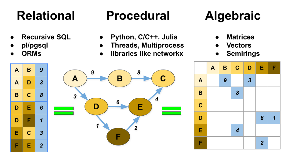
We can see here there are three distinct form of graph analysis, relational, procedural, and algebraic. OneSparse aims to unify all three models so that you have maximum flexibility when you process your graph data. Combined workflows, like ETL processing with SQL, traditional per-edge style traversal with Python, and high performance graph analysis with algebra are possible and encouraged.
Using the relatively new Table Access Method (TAM) API, we are working to have automatic graph updates happen completely behind the scenes, no matrices or vectors, just edge tables and super-fast algorithms. While you can always drop "down to the algebra" if you want to, this will provide a much simpler interface for users who already have the algorithms and data in hand.
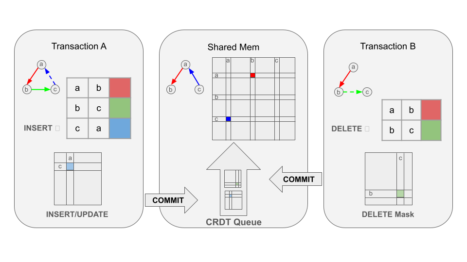
In the next release, we will store TAM-backed graphs in shared memory, avoiding loading costs to enable very high performance traversal with high query throughput. Insert, updates and other modifications of the matrix will be performed asynchronously using CRDT Graph semantics for near-zero latency commits with eventual consistency to the graph, while still ensuring strong ACID consistency at the table level.
OneSparse is a very early product, and we encourage you to try it out and send us feedback, but do expect some rapid changes and advancements over the next few months.